Introduction
In any measurement system, you cannot capture what you cannot distinguish. Dynamic range defines the usable window between the loudest signal a DAQ system can handle and the quietest it can resolve—a specification that directly determines whether your equipment can detect the microvolt-level defect signatures that separate good parts from scrap.
Narrow that window through poor specification choices, and the result is clipped signals, buried noise, and unreliable data. According to research on high-precision ADC signal chains, practical dynamic range in commercial 24-bit DAQ systems typically delivers 100–118 dB rather than the theoretical 146 dB—a gap driven by thermal noise, power supply coupling, and front-end electronics limitations.
This article covers:
- What dynamic range actually means in a DAQ context
- The physical factors that govern it in real hardware
- How to calculate and verify it for your application
- Where misapplication causes measurement failures in the field
Key Takeaways
- Dynamic range (in dB) is the ratio between the largest signal a DAQ system can accurately measure and the smallest it can distinguish from noise
- In practice, clipping sets the upper limit while noise floor, ADC resolution, and spurious artifacts define the lower bound
- ADC bit depth sets a theoretical ceiling; 24-bit systems achieve 100–118 dB in practice, not the theoretical 146 dB
- Gain, input range, and bandwidth settings determine how much of that available dynamic range you actually capture
- Mismatched dynamic range leads to missed defects, bad pass/fail calls, and unreliable baseline data in production testing
What Dynamic Range Means in a DAQ System
Dynamic range is the ratio of the full-scale input amplitude (V_FS) to the RMS system noise floor (V_N), typically expressed in decibels using DR = 20 × log10(V_FS / V_N). This is not a passive label but a hard boundary on what the system can and cannot resolve. If your signal falls below the noise floor, it cannot be measured. If it exceeds the full-scale range, it clips and produces distorted, unusable data.
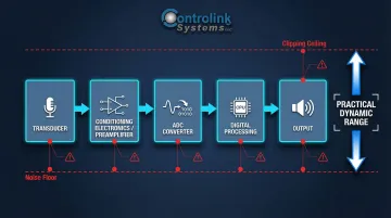
Dynamic range is a system-level design parameter, not simply an ADC specification. It is a property of the entire signal chain—from transducer and conditioning electronics through ADC conversion to digital processing. The weakest link in that chain determines the practical dynamic range you can achieve, regardless of how capable your ADC might be on paper.
Both limits have separate causes and separate engineering controls:
- Upper limit: set by the system's full-scale input or clipping level — exceed it and data distorts
- Lower limit: the noise floor — fall below it and the signal disappears into noise
Understanding how each limit behaves is what drives proper system configuration. It also explains why dynamic range cannot be evaluated without knowing the measurement bandwidth.
Broadband vs. Narrowband Dynamic Range
Dynamic range is frequency-bandwidth dependent. In well-designed systems, noise approximates white noise — distributed evenly across frequency. Narrowing the analysis bandwidth through FFT or narrowband filtering reduces the effective noise floor and increases usable dynamic range.
When moving from broadband time-domain measurements to narrowband FFT analysis, the system achieves a "processing gain." The theoretical FFT noise floor drops by:
10 × log10(fs / (2 × BW))
where fs is the sampling rate and BW is the bandwidth of interest. This is why a 24-bit system can report meaningfully different dynamic ranges in broadband vs. narrowband analysis modes.
That frequency dependence makes bandwidth context mandatory in any dynamic range specification. A figure quoted without it is incomplete — and in practice, it's the most common reason a system that looked right on a datasheet fails to resolve the signals you actually need to measure.
What Limits Dynamic Range: Upper and Lower Boundaries
Every element of the signal chain contributes a limitation. The practical dynamic range of the full system is bounded by the weakest-performing element, not the best. Understanding both boundaries — the noise floor below and the saturation ceiling above — is what separates a well-configured DAQ system from one that loses data at the extremes.
Lower Limit: Noise Floor and Related Artifacts
The noise floor is the absolute lower limit—signals buried below it cannot be measured. The noise floor is a composite of several contributors:
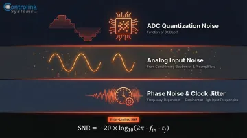
- ADC quantization noise — a function of bit depth
- Analog input noise — from conditioning electronics and preamplifiers
- Spurious artifacts — from power supply coupling or clock interference
Phase noise is an additional lower-limit factor in precision dynamic measurements. Oscillator instability creates frequency sidebands that raise the effective noise floor near a carrier frequency, reducing the usable dynamic range for small signals adjacent to large ones. At high input frequencies, clock phase noise (aperture jitter) supersedes quantization noise as the primary SNR limiter.
The theoretical limit on SNR resulting from clock jitter is calculated as SNR = -20 × log10(2π fin tj), where fin is the input frequency and tj is the RMS jitter. This means that as input frequencies increase, even sub-picosecond jitter can severely degrade the dynamic range of a 24-bit system.
Upper Limit: Clipping, Compression, and Spurious Products
The upper limit is reached when input signal amplitude causes the analog front end or ADC to saturate (clip), producing distorted, non-linear output. The 1 dB compression point characterizes where gain linearity breaks down: specifically, the output power level at which an amplifier's gain has compressed by 1 dB from its ideal linear value.
Compression generates spurious products—harmonic distortion and intermodulation products—that appear as false signals in the measurement data. Spurious-free dynamic range (SFDR) is the relevant metric when spurious artifacts, not noise, are the primary limiting factor. SFDR is defined as the ratio of the RMS amplitude of the fundamental carrier frequency to the RMS value of the next largest noise or harmonic distortion component, reported in dBc (relative to the carrier).
Additional practical limiters include:
- Cross-talk between adjacent channels
- ADC non-linearity (uneven quantization steps)
- Aliasing from signals above the Nyquist frequency
- DSP chain precision limitations
A 24-bit ADC yields a theoretical dynamic range of approximately 146 dB, yet commercial 24-bit DAQ systems typically deliver 100–118 dB in practice. The gap is driven by thermal noise, analog front-end electronics noise, reference voltage noise, and electromagnetic interference.
Real device specs illustrate this clearly:
- NI PXIe-4497: 114 dB dynamic range
- NI 4461: 118 dB dynamic range
- NI 9234 C-Series: 102 dB dynamic range
How Dynamic Range Is Calculated and Expressed in dB
The dB calculation is straightforward: DR (dB) = 20 × log10(V_FS / V_N). The log scale compresses large ratios into manageable numbers. A 120 dB dynamic range means the largest measurable signal is one million times larger in amplitude than the smallest detectable signal—a span that would be impossible to visualize or work with on a linear scale.
The theoretical relationship between ADC bit depth and dynamic range uses the rule of thumb: DR ≈ 6.02 × N + 1.76 dB, where N is the number of bits. Based on this formula:
- A 16-bit ADC yields approximately 98 dB theoretical dynamic range
- A 24-bit ADC yields approximately 146 dB theoretical dynamic range
Real-world measurements fall short of these ceilings because the formula assumes an ideal ADC with no thermal noise, no analog conditioning degradation, and no spurious artifacts. In practice, every real system introduces noise and distortion that pull measured performance below the theoretical limit.
How Gain Settings Affect Usable Dynamic Range
Gain settings directly determine how much of the ADC's available bit depth gets applied to the actual signal. Applying an appropriate gain narrows the input range to match the signal amplitude, so the converter uses more resolution where it matters. This improves measurement precision within the dynamic range window.
This is fundamentally different from screen scaling, which changes display appearance without affecting actual resolution. Setting the input range far larger than the expected signal amplitude wastes available ADC resolution and shrinks the usable dynamic range for that measurement.
Specifying, Measuring, and Validating Dynamic Range
Dynamic range is both a design-time specification (from datasheets, rated input range, and noise figures) and an operational parameter that must be verified against real signal conditions. Rated values represent best-case scenarios under controlled lab conditions. Field conditions—temperature variation, grounding issues, cable routing, and EMI—will typically reduce practical dynamic range below datasheet values.
Standard Measurement Methods
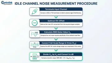
The idle channel noise approach is the most common baseline test:
- Terminate the input channel (e.g., with a 50 Ω terminator)
- Subtract the DC offset from the acquired signal
- Calculate the RMS value of the remaining noise signal (V_N)
- Convert the full-scale input range to Vrms (V_FS)
- Divide V_FS by V_N and convert the ratio to dB
The industry standard method uses a high-quality -60 dBFS input tone rather than a terminated channel. This approach is superior because some ADCs artificially mute their outputs when they detect a completely dead (grounded) input, which falsely inflates the dynamic range measurement. The -60 dBFS tone keeps the ADC active, quantifying the true distortion and noise present when a low-level signal is processed.
NI-based DAQ platforms include built-in tools — LabVIEW's Mean VI, RMS VI, and Logarithm Base 10 functions — that let engineers programmatically characterize dynamic range in the actual deployment environment, not just on paper. Controlink Systems configures and deploys these NI platforms for high-speed process monitoring, vibration analysis, and end-of-line testing.
Laboratory vs. Field Validation
Dynamic range should be re-verified after installation, particularly for multichannel systems where cross-talk and grounding configurations can degrade performance. Several field conditions commonly reduce measured dynamic range below datasheet values:
- Thermal drift: Temperature variations cause baseline drift and alter amplifier offset/gain errors (source)
- EMI pickup: Unshielded cables act as antennas, capturing radiative interference from nearby motors or fluorescent lights
- Grounding loops: Multichannel systems with inconsistent ground references introduce common-mode noise that narrows usable range
Practical Implications: Mismatched Dynamic Range and Common Mistakes
When dynamic range is too narrow for the application, large signals clip and produce distorted data while small signals disappear into the noise floor. Both failure modes corrupt your measurements before any analysis even begins.
In manufacturing and vibration testing environments, this translates directly to missed defects, false pass/fail results, and corrupted baseline measurements. These errors often go undetected at the source but propagate through downstream analysis and compromise product quality.
Most Common Practical Mistakes
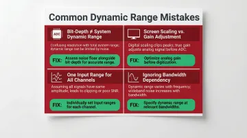
- Bit-depth ≠ system dynamic range: A 24-bit ADC does not deliver 146 dB in practice. Thermal noise, power supply coupling, and front-end electronics reduce real-world performance to 100–118 dB.
- Screen scaling is not gain adjustment: Changing display appearance does nothing to measurement resolution. Only reconfiguring input range to match signal amplitude maximizes available ADC codes.
- One input range for all channels: In multichannel systems with varying amplitudes, a single range wastes resolution on weak channels and risks clipping on strong ones. Configure each channel independently.
- Ignoring bandwidth dependency: Narrowband and broadband dynamic range specs are not interchangeable. A system that meets spec on a narrowband measurement can fail outright on broadband signals.
The Consequence of Over-Ranging
Of the mistakes above, over-ranging is both the most common and the easiest to fix. Setting the input range far larger than the expected signal amplitude wastes ADC resolution and shrinks usable dynamic range for that measurement.
The correct approach: select the highest gain (narrowest input range) that captures the full signal without clipping. This applies equally to hardware configuration and software gain settings. The result is more ADC codes representing the signal, better measurement resolution, and reduced quantization noise.
Frequently Asked Questions
What is the purpose of dynamic range in a data acquisition system?
Dynamic range defines the span of signal amplitudes a DAQ system can accurately capture simultaneously—from the smallest detectable signal above the noise floor to the largest before clipping occurs. It directly determines whether the system is suitable for a given measurement application, particularly when both large and small signals must be measured in the same acquisition.
What does a 120 dB dynamic range mean for a data acquisition system?
120 dB means the maximum measurable signal is one million times larger in amplitude than the minimum detectable signal. The system can handle very large and very small signals simultaneously without losing resolution at either extreme—making it well-suited for vibration analysis where large resonances coexist with small defect signatures.
How do you calculate dynamic range in dB for a data acquisition system?
Use the formula DR = 20 × log10(V_FS / V_N), where V_FS is the full-scale input amplitude in Vrms and V_N is the RMS noise floor. The idle channel noise method (terminating the input, measuring RMS noise, then comparing to full-scale range) is the standard practical approach for characterizing real systems.
How does ADC bit depth affect dynamic range?
ADC bit depth sets the theoretical ceiling using the relationship DR ≈ 6.02 × N + 1.76 dB. A 24-bit ADC has a theoretical maximum of approximately 146 dB, but real systems typically achieve 100–110 dB due to analog conditioning noise, non-linearity, and other signal chain imperfections.
What is the difference between dynamic range and spurious-free dynamic range (SFDR)?
Dynamic range spans from the noise floor to the clipping level, while SFDR is the difference between the fundamental signal and the largest spurious (distortion) product. SFDR is the more relevant metric when compression-generated artifacts, rather than noise, are the primary limitation on measurement accuracy—particularly in applications measuring small signals near large ones.
Why does narrowband analysis improve dynamic range?
System noise is distributed across frequency, so reducing analysis bandwidth (via FFT with fewer lines or narrower resolution bandwidth) reduces the noise integrated into the measurement. This lowers the noise floor and increases usable dynamic range within that band—a principle Delta-Sigma ADCs exploit through oversampling and digital decimation.